Objective
Nearly four years after writing a blog post about recreating R figures in ODV I had someone reach out to me expressing interest in adding a bathymetry layer over the interpolated data. It’s always nice to know that these blog posts are being found useful for other researchers. And I have to admit I’m a bit surprised that the code still runs 4 years later. Especially considering that it uses the tidyverse which is notorious for breaking backwards compatibility. In order to demonstrate the overlaying of bathymetry data on a CTD transect we will need to use a different dataset than in the previous blog post. One may use any data one would like, but for this blog I went to this shiny app to extract some data from the coast of South Africa. Specifically I filtered for temperature data from November 1990 at all depths. We won’t go back over the theory for recreating the ODV figure in this blog post, so please revisit that for a recap as necessary. Below I will show two of the necessary steps to get interpolated CTD data before we begin on the bathymetry mask.
# Load libraries
library(tidyverse)
library(lubridate)
library(reshape2)
library(MBA)
library(mgcv)
library(marmap)
library(FNN)

# The transects in this dataset do not have an ID column
# So we manually select the first transect (rows 1 - 12)
# This is then used as a mask to select all depths for these pixels
# We will also use these unique lon/lat coords for bathymetry points
ctd_mask <- read_csv("../../static/data/CTD_transect.csv") %>%
  select(lon, lat) %>%
  slice(1:12) %>%
  unique()

# Load and screen data
  # For ease I am only using monthly means
  # and depth values rounded to 10 metres
ctd <- read_csv("../../static/data/CTD_transect.csv") %>%
  mutate(depth = -depth) %>%  # Correct for plotting
  right_join(ctd_mask, by = c("lon", "lat")) %>%
  select(lon, lat, depth, temp)

# Manually extracted hexidecimal ODV colour palette
ODV_colours <- c("#feb483", "#d31f2a", "#ffc000", "#27ab19", "#0db5e6", "#7139fe", "#d16cfa")

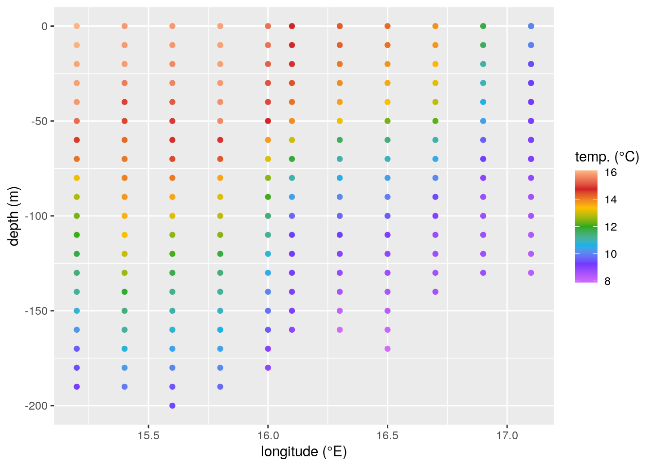
# Create quick scatterplot
ggplot(data = ctd, aes(x = lon, y = depth)) +
  geom_point(aes(colour = temp)) +
  scale_colour_gradientn(colours = rev(ODV_colours)) +
  labs(y = "depth (m)", x = "longitude (°E)", colour = "temp. (°C)")

Figure 1: A non-interpolated scatterplot of our temperature (°C) data shown as a function of depth (m) over longitude (°E).
It looks like we have a nice little upwelling signal coming through at the coast. It will be interesting to see how the interpolation handles that. We’ll quickly run the interpolation and then get to the bathymetry overlay. Note that these data are not on a straight latitude transect, but we are not going to worry about that in this blog post.
# Now we may interpolate the data
# NB: The columns that mba.surf() will interpolate are the X, Y, Z values in that order
ctd_mba <- mba.surf(ctd[c("lon", "depth", "temp")], no.X = 300, no.Y = 300, extend = T)
dimnames(ctd_mba$xyz.est$z) <- list(ctd_mba$xyz.est$x, ctd_mba$xyz.est$y)
ctd_mba <- melt(ctd_mba$xyz.est$z, varnames = c('lon', 'depth'), value.name = 'temp') %>%
  filter(depth < 0) %>%
  mutate(temp = round(temp, 1))

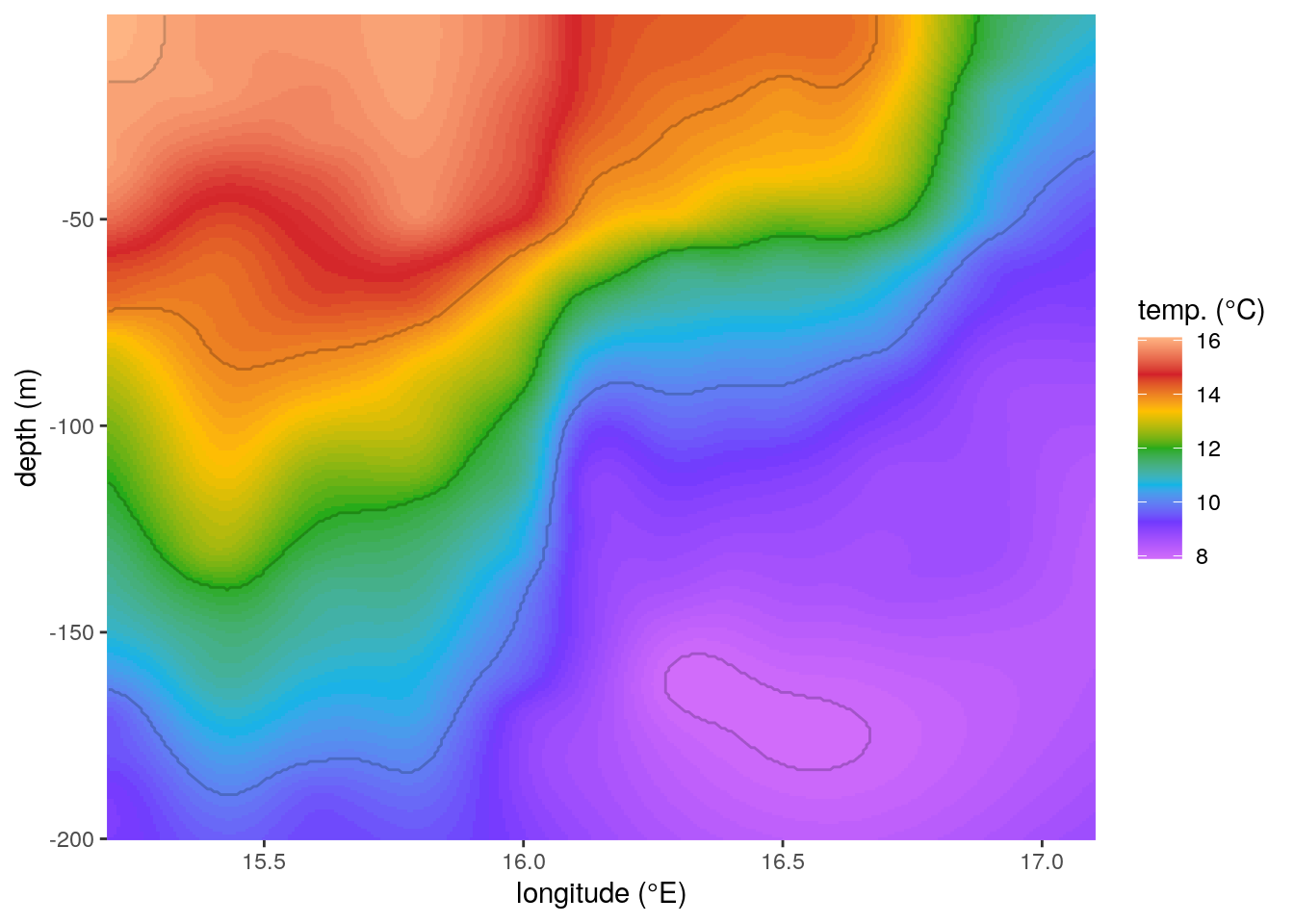
# Finally we create our gridded result
ggplot(data = ctd_mba, aes(x = lon, y = depth)) +
  geom_raster(aes(fill = temp)) +
  geom_contour(aes(z = temp), binwidth = 2, colour = "black", alpha = 0.2) +
  geom_contour(aes(z = temp), breaks = 20, colour = "black") +
  scale_fill_gradientn(colours = rev(ODV_colours)) +
  labs(y = "depth (m)", x = "longitude (°E)", fill = "temp. (°C)") +
  coord_cartesian(expand = F)

Figure 2: The same temperature (°C) profiles seen in Figure 1 with the missing values filled in with multilevel B-splines.
Bathymetry
The interpolation seems to have done a decent job of acknowledging the upwelling signal. It may be possible to tweak the interpolation more, as desired, but I’m happy enough with it for the purposes of this post. We are going to skip over the step to cut out the artefacts at the bottom of the figure where there are not data points because we are rather going to just overlay our bathymetry mask. First we will download the bathymetry data. Then we find the points that are closest to our CTD transect. These will then be used for the grey overlay at the bottom of the figure.
# Bathymetry within transect bounding box
bathy <- getNOAA.bathy(lon1 = min(ctd$lon), lon2 = max(ctd$lon),
                       lat1 = min(ctd$lat), lat2 = max(ctd$lat),
                       resolution = 5) # Larger numbers for coarser data

# Convert bathy object to a data.frame for easier use
bathy_df <- data.frame(lon_b = as.numeric(rownames(bathy)),
                       lat_b = as.numeric(colnames(bathy)),
                       depth = as.numeric(bathy)) %>%
  mutate(bathy_idx = 1:n()) # Used for merging CTD and bathy data

# Find nearest points to transect data
ctd_mask <- ctd_mask %>%
  mutate(bathy_idx = as.vector(knnx.index(as.matrix(bathy_df[,c("lon_b", "lat_b")]),
                                           as.matrix(ctd_mask[,c("lon", "lat")]), k = 1))) %>%
  left_join(bathy_df, by = "bathy_idx")

# Manually create bottom of the bathy mask polygon
bathy_mask <- data.frame(lon = c(ctd_mask$lon, rev(ctd_mask$lon)),
                         depth = c(ctd_mask$depth, rep(min(ctd_mask$depth), nrow(ctd_mask))))

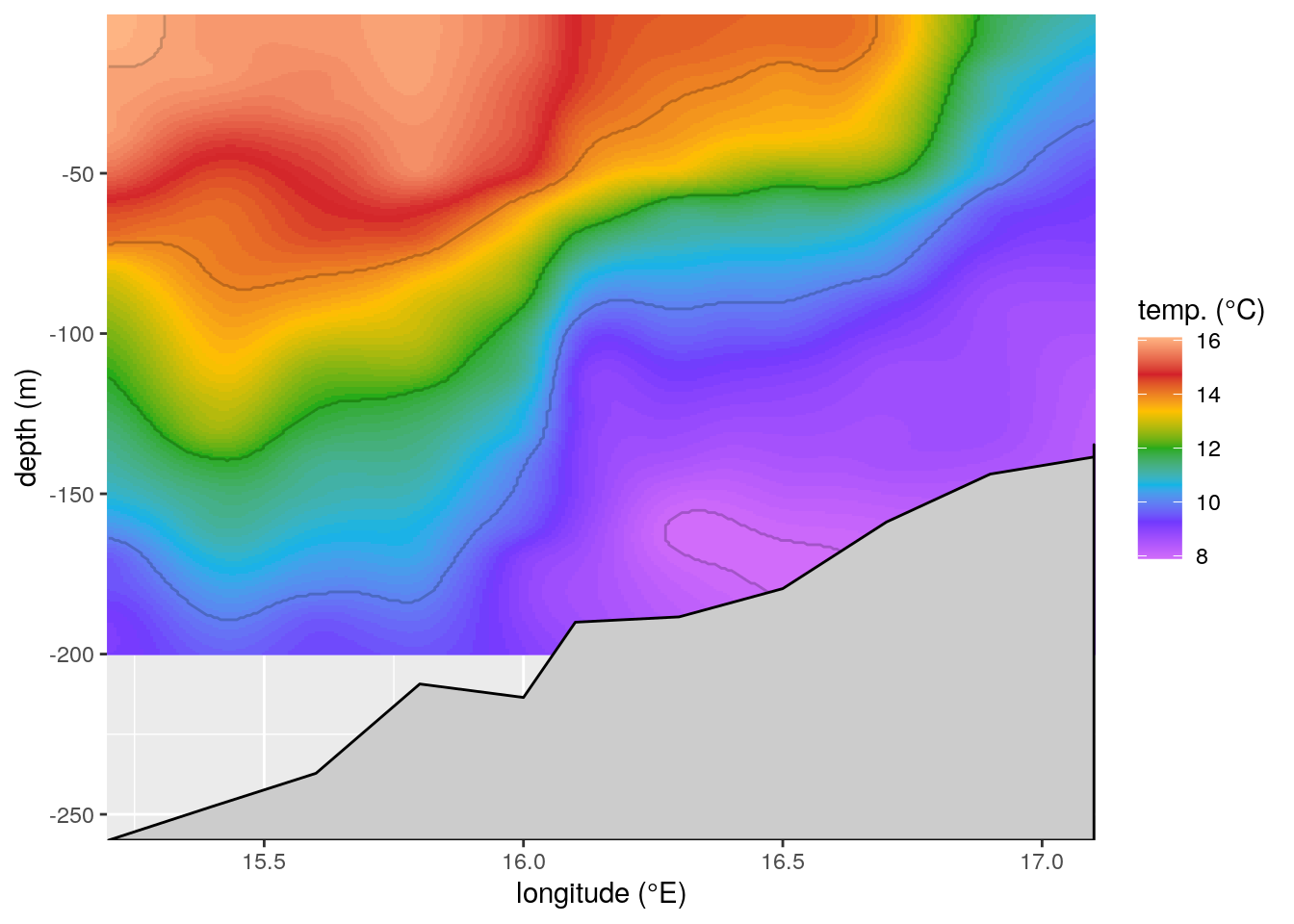
# We may now use that bathy mask for our final figure
ggplot(data = ctd_mba, aes(x = lon, y = depth)) +
  geom_raster(aes(fill = temp)) +
  geom_contour(aes(z = temp), binwidth = 2, colour = "black", alpha = 0.2) +
  geom_contour(aes(z = temp), breaks = 20, colour = "black") +
  geom_polygon(data = bathy_mask, fill = "grey80", colour = "black") +
  scale_fill_gradientn(colours = rev(ODV_colours)) +
  labs(y = "depth (m)", x = "longitude (°E)", fill = "temp. (°C)") +
  coord_cartesian(expand = F)

Figure 3: The same temperature (°C) profiles seen in Figure 2 with the bathymetry values overlaid.
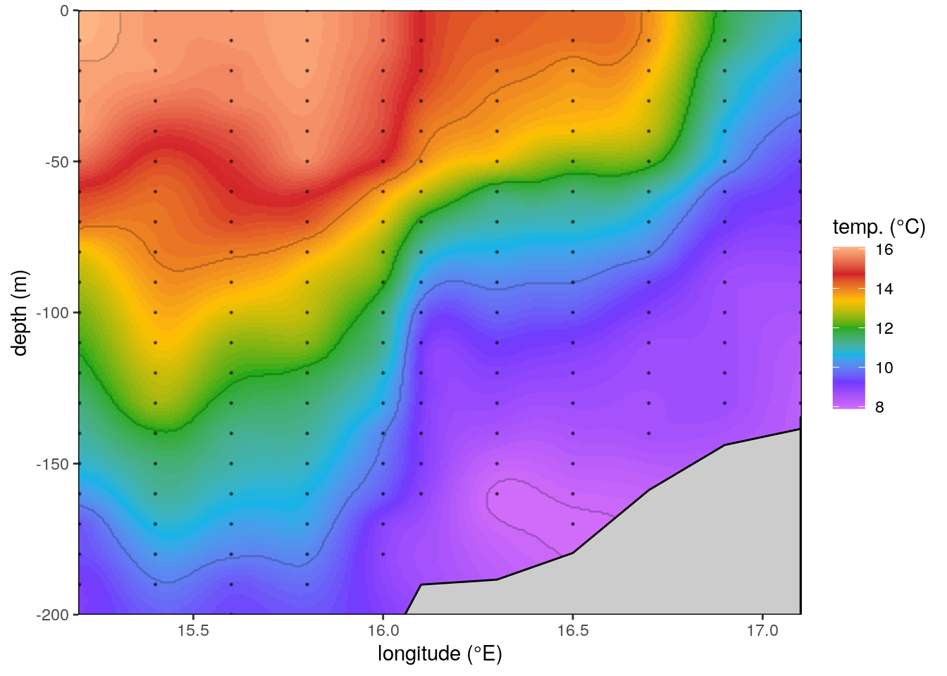
Unfortunately in this example there is a bit of blank space in the bottom left of the plot because the CTD casts do not go deeper than 200 m, and the interpolation doesn’t fill in values outside of the rectangular box dictated by the X (lon) and Y (depth) values. A cheeky workaround for this issue would be to simply crop the figure to the bottom of the interpolated data, and not the bathymetry.
# We may now use that bathy mask for our final figure
ggplot(data = ctd_mba, aes(x = lon, y = depth)) +
  geom_raster(aes(fill = temp)) +
  geom_contour(aes(z = temp), binwidth = 2, colour = "black", alpha = 0.2) +
  geom_contour(aes(z = temp), breaks = 20, colour = "black") +
  geom_polygon(data = bathy_mask, fill = "grey80", colour = "black") +
  geom_point(data = ctd, aes(x = lon, y = depth),
             colour = 'black', size = 0.2, alpha = 0.4, shape = 8) +
  scale_fill_gradientn(colours = rev(ODV_colours)) +
  labs(y = "depth (m)", x = "longitude (°E)", fill = "temp. (°C)") +
  coord_cartesian(expand = F, ylim = c(-200, 0)) +
  theme(panel.border = element_rect(fill = NA, colour = "black"))
 Figure 4: The plotting area cropped to the interpolated data, rather than the bathymetry mask. Also shown with black dots are the original CTD data.
Summary
In this tutorial we have seen how to plot a bathymetry overlay that matches the lon/lat coordinates of the CTD casts. I’m sure there is a way to force the interpolation to fill in values at a greater depth to match the bathymetry, but the focus of this blog was on adding the bathymetry mask itself, and I think we have addressed this issue. The workflow outlined above has a couple of bumps in it, but should be adaptable to a range of applications.