Transects

Preface

This week I have expanded the coastR package with the inclusion of a function that calculates the angle of the heading for alongshore or shore-normal transects. The rest of this blog post is the vignette that I’ve written detailing the set of this function. Next week I’ll likely be taking a break from coastR development to finally create a package for the SACTN dataset. That is a project that has been in the works for a loooong time and it will be good to finally see a development release available to the public.

Overview

There are a number of reasons why one would want to calculate transects along or away from a coastline. Examples include: finding the fetch across an embayment, finding the coordinates of a point 200 km from the coast, finding the appropriate series of SST pixels along/away from the coast, (or if one is feeling particular feisty) the creation of shape files for a given area away from the coast. The function that we will be introducing here does none of these things. What the transects() function does do is calculate the angle of the heading along or away from the coast against true North, which is then the basis for all of the other fancy things one may want to do. Baby steps people. Baby steps.

# devtools::install_github("robwschlegel/coastR") # Install coastR
library(coastR)
library(dplyr)
library(ggplot2)
library(gridExtra)
library(geosphere)

Sample locations

For this vignette we will re-use the same coastlines as those created for the sequential sites vignette. The ordering of the sites remains jumbled up to demonstrate that transects() does not require orderly data. Should one want to order ones site list before calculating transect headings it is possible to do so with seq_sites(). This is of course a recommended step in any workflow.

# Cape Point, South Africa
cape_point <- SACTN_site_list %>% 
  slice(c(31, 22, 26, 17, 19, 21, 30)) %>% 
  mutate(order = 1:n())

# South Africa
south_africa <- SACTN_site_list %>% 
  slice(c(1,34, 10, 20, 50, 130, 90)) %>% 
  mutate(order = 1:n())

# Baja Peninsula, Mexico
baja_pen <- data.frame(
  order = 1:7,
  lon = c(-116.4435, -114.6800, -109.6574, -111.9503, -112.2537, -113.7918, -114.1881),
  lat = c(30.9639, 30.7431, 22.9685, 26.9003, 25.0391, 29.4619, 28.0929)
)

# Bohai Sea, China
bohai_sea <- data.frame(
  order = 1:7,
  lon = c(122.0963, 121.2723, 121.0687, 121.8742, 120.2962, 117.6650, 122.6380),
  lat = c(39.0807, 39.0086, 37.7842, 40.7793, 40.0691, 38.4572, 37.4494)
)

Transects

With our site lists created we now want to see what the correct headings for alongshore and shore-normal transects are for our sites. We will also demonstrate what happens when we increase the spread used in the calculation and also how the inclusion of island masks affects the angle of the headings.

# Cape Point, South Africa
cape_point_along <- transects(cape_point, alongshore = T)
cape_point_away <- transects(cape_point)

# South Africa
south_africa_along <- transects(south_africa, alongshore = T)
south_africa_away <- transects(south_africa)
  # NB: Note here the use of the `spread` argument
south_africa_along_wide <- transects(south_africa, alongshore = T, spread = 30)
south_africa_away_wide <- transects(south_africa, spread = 30)

# Baja Peninsula, Mexico
baja_pen_along <- transects(baja_pen, alongshore = T)
baja_pen_away <- transects(baja_pen)
  # NB: Note here the use of the `coast` argument
baja_pen_island <- transects(baja_pen, coast = FALSE)

# Bohai sea, China
bohai_sea_along <- transects(bohai_sea, alongshore = T)
bohai_sea_away <- transects(bohai_sea)

Visualise

Now that the correct headings have been calculated for our alongshore and shore-normal transects let’s visualise them with ggplot. First we will create a function that does this in order to keep the length of this vignette down.

# Create base map
world_map <- ggplot() + 
  borders(fill = "grey40", colour = "black")

# Create titles
titles <- c("Alongshore", "Shore-normal", "Islands")

# Plotting function
plot_sites <- function(site_list, buffer, title_choice, dist){
  
  # Find the point 200 km from the site manually to pass to ggplot
  heading2 <- data.frame(geosphere::destPoint(p = select(site_list, lon, lat),  
                                              b = site_list$heading, d = dist))
  
  # Add the new coordinates tot he site list
  site_list <- site_list %>% 
    mutate(lon_dest = heading2$lon,
           lat_dest = heading2$lat)
  
  # Visualise
  world_map +
    geom_segment(data = site_list, colour = "red4", 
                 aes(x = lon, y = lat, xend = lon_dest, yend = lat_dest)) +
    geom_point(data = site_list, size = 3, colour = "black", aes(x = lon, y = lat)) +
    geom_point(data = site_list, size = 3, colour = "red", aes(x = lon_dest, y = lat_dest)) +
    coord_cartesian(xlim = c(min(site_list$lon - buffer), 
                             max(site_list$lon + buffer)),
                    ylim = c(min(site_list$lat - buffer), 
                             max(site_list$lat + buffer))) +
    labs(x = "", y = "", colour = "Site\norder") +
    ggtitle(titles[title_choice])
}

Cape Point, South Africa

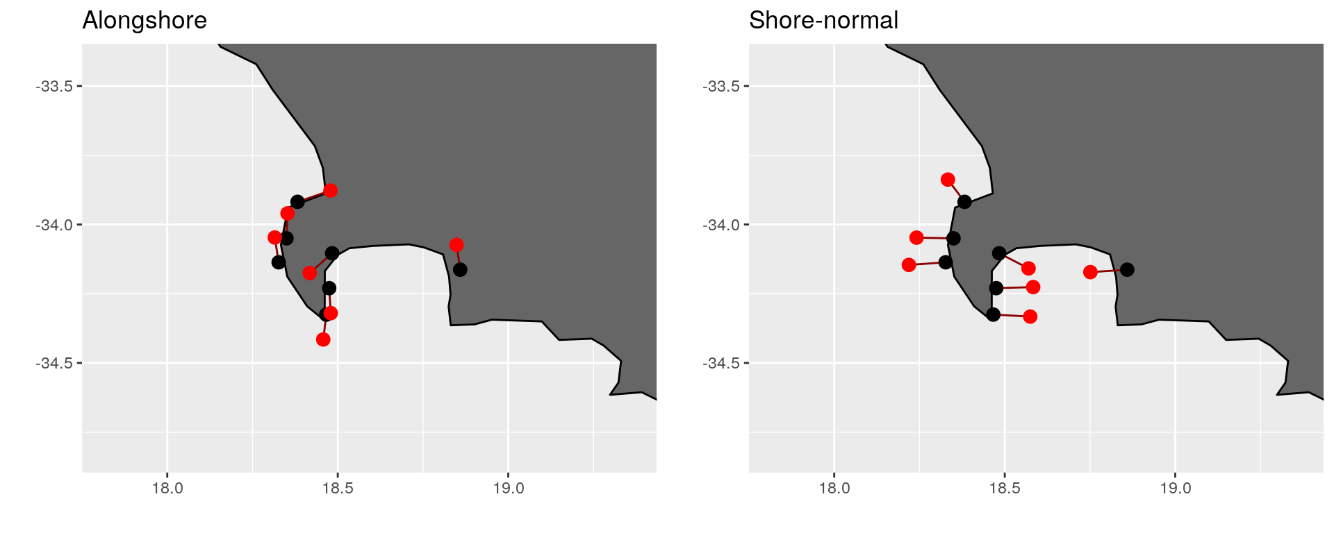
The transect() function is designed to work well at small scales by default. We may see this here with the effortlessness of plotting transects around a peninsula and then across an embayment in one go.

cape_point_along_map <- plot_sites(cape_point_along, 0.5, 1, 10000)
cape_point_away_map <- plot_sites(cape_point_away, 0.5, 2, 10000)
grid.arrange(cape_point_along_map, cape_point_away_map, nrow = 1)

South Africa

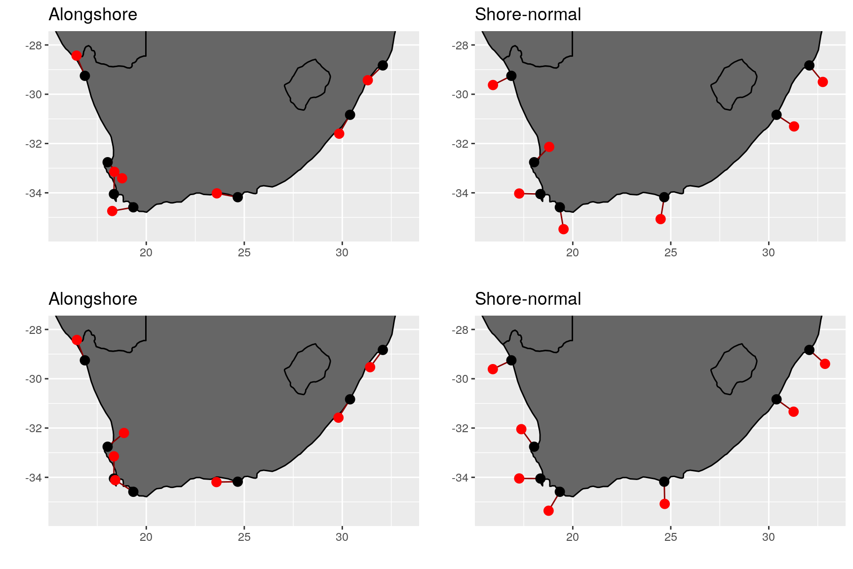
The intentions one may have for calculating shore-normal transects will differ depending on ones research question. If one is interested in visualising the convolutions of a coastline at a sub-meso-scale then the default spread of the transect() function is probably the way to go, as shown above. If however one is interested in seeing the shore-normal transects broadly for the coastline of an entire country it is likely that one will want to greatly expand the spread of coastline used to calculate said transects. In the figure below we may see how changing the spread of the coastline considered for the transects changes the results. The top row shows the transects resulting from the narrow default spread, while the bottom row shows the results of using a much wider spread for the calculation. Note particularly how the transect changes at St. Helena Bay and Gansbaai (second and fourth sites from the top left), as well as a general smoothing of all of the other transects. This is due to the sensitivity of the function. The St. Helena Bay and Gansbaai sites lay within embayments; therefore, the shore-normal transects that would come out directly from these sites will not follow the general contour of the coastline of South Africa. Should we be interested in the “bigger picture” we must increase the spread argument in transects(). This may require some trial and error for particularly difficult coastlines before a satisfactory result is produced, but it is certainly still faster than running the calculations by hand. Should small scale accuracy along part of the coast, and broader accuracy elsewhere be required, one must simply divide the site list into the different sections and run transects() on each subset with the desired spread.

south_africa_along_map <- plot_sites(south_africa_along, 1, 1, 100000)
south_africa_away_map <- plot_sites(south_africa_away, 1, 2, 100000)
south_africa_along_wide_map <- plot_sites(south_africa_along_wide, 1, 1, 100000)
south_africa_away_wide_map <- plot_sites(south_africa_away_wide, 1, 2, 100000)
grid.arrange(south_africa_along_map, south_africa_away_map, 
             south_africa_along_wide_map, south_africa_away_wide_map, nrow = 2)

Baja Peninsula, Mexico

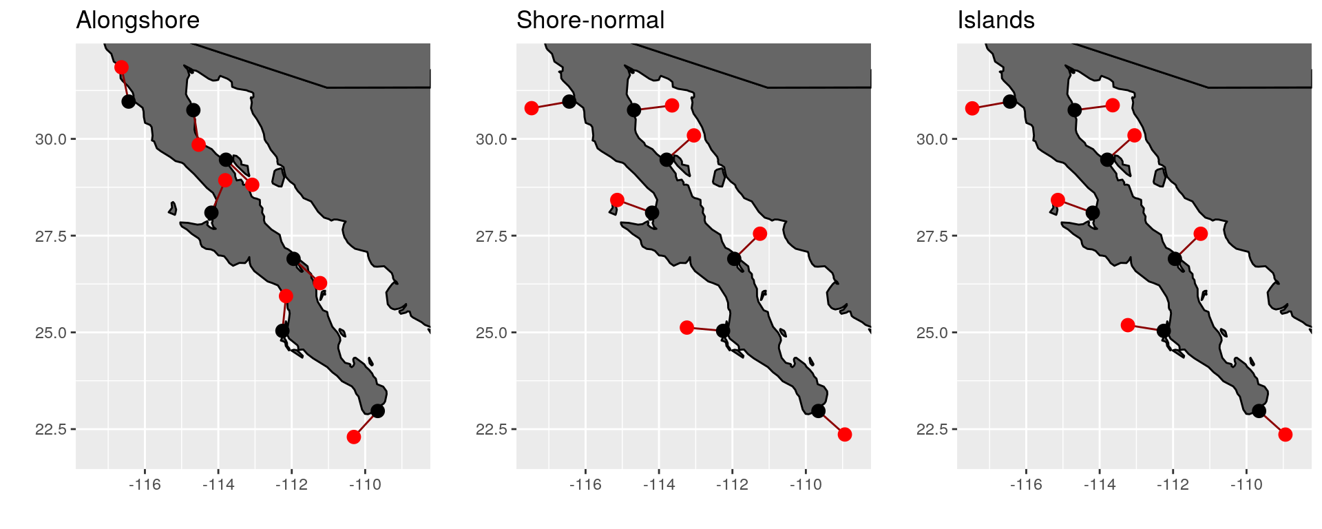
In the following figure we see how the inclusion of islands affects the results of our transects. The first site up from the tip of the peninsula on the left-hand side is on an island. Note the minor adjustment to the transect when the island mask is used for the calculation. In this case it’s not large, but in other instances it may be massive. By default island masks are removed and it is our advice that they not be used unless extreme caution is observed.

baja_pen_along_map <- plot_sites(baja_pen_along, 1, 1, 100000)
baja_pen_away_map <- plot_sites(baja_pen_away, 1, 2, 100000)
baja_pen_island_map <- plot_sites(baja_pen_island, 1, 3, 100000)
grid.arrange(baja_pen_along_map, baja_pen_away_map, baja_pen_island_map, nrow = 1)

Bohai Sea, China

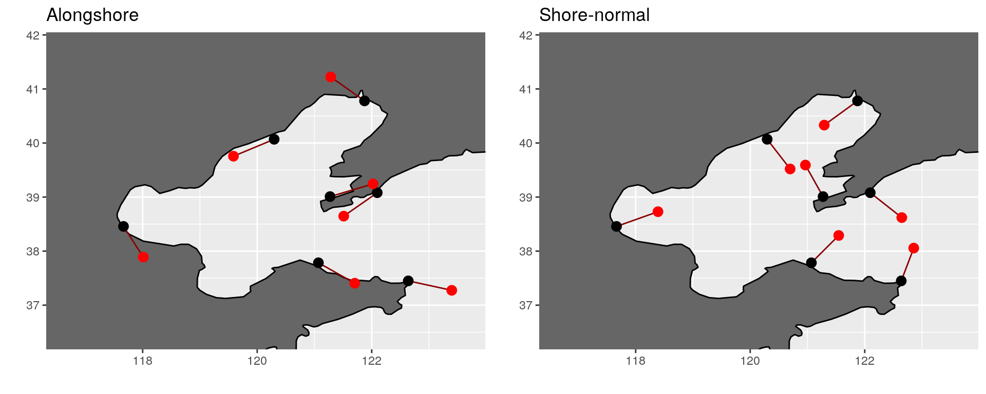
This figure serves as a good visualisation for just how localised the coastline is that is used to calculate the shore-normal transects. Note how the alongshore transects look a little dodgy, but when shown as shore-normal transects everything works out. This is something to consider if one is interested in calculating alongshore transects rather than shore-normal transects. For alongshore transects that show more fidelity for coastal direction it is advisable to increase the spread argument.

bohai_sea_along_map <- plot_sites(bohai_sea_along, 1, 1, 70000)
bohai_sea_away_map <- plot_sites(bohai_sea_away, 1, 2, 70000)
grid.arrange(bohai_sea_along_map, bohai_sea_away_map, nrow = 1)

Conclusion

As we may see in the previous example figures, the transect() function tends to work better by default at smaller scales. This was an intentional decision as it is much more accurate when scaling the function up for larger coastal features than when scaling it down for smaller ones.

The calculation of the heading for alongshore and shore-normal transects is rarely the end goal itself. One then generally wants to find specific points from the coastline along the transects that have been determined. This is done in the code above within the plot_sites() function created within this vignette, but the process is not detailed specifically. How to do more elaborate things with transects will be explained with the following functions to be added to coastR. This will include how to draw coastal polygons based on distance and bathymetry.