Objective
In South Africa there are a range of idioms for different time frames in which someone may (or may not) do something. The most common of these are: ‘now’, ‘just now’, and ‘now now’. If one were to Google these sayings one would find that there is general agreements on how long these time frames are, but that agreement is not absolute.

This got me to wondering just how much disagreement there may be around the country. And more specifically I wanted to know how these times changed between specific locations. If one is interested in contributing to the survey, it may be taken here. To avoid too much confusion with the answers that could be given, specific times were provided to the participants in a multiple choice format. These times (minutes) were: 5, 15, 30, 60, 120, 300.
Data prep
The survey data are downloaded from Google Forms rather easily as a .csv file, so that’s nice. Unfortunately, the way in which one sets up the survey for humans is difficult for R to understand so we need quite a bit of processing after we load the data.
library(tidyverse)
library(ggpubr)
library(broom)

survey <- read_csv("../../static/data/SA Time Survey.csv", skip = 1, col_types = "cccccc",
                   col_names = c("time", "just now", "now now", "now", "province", "city")) %>%
  select(-time) %>%
  mutate(`just now` = as.numeric(sapply(strsplit(`just now`, " "), "[[", 1)),
         `now now` = as.numeric(sapply(strsplit(`now now`, " "), "[[", 1)),
         `now` = as.numeric(sapply(strsplit(`now`, " "), "[[", 1)),
         province = gsub("Kzn", "KZN", province),
         province = gsub("GP", "Gauteng", province),
         province = as.factor(province),
         city = as.factor(city))

# Check that city and province names are all lekker
# levels(survey$province)
# levels(survey$city)

# Create a long version for easier stats
survey_long <- survey %>%
  gather(key = "saying", value = "minutes", -province, -city) %>%
  na.omit()
Participant locations
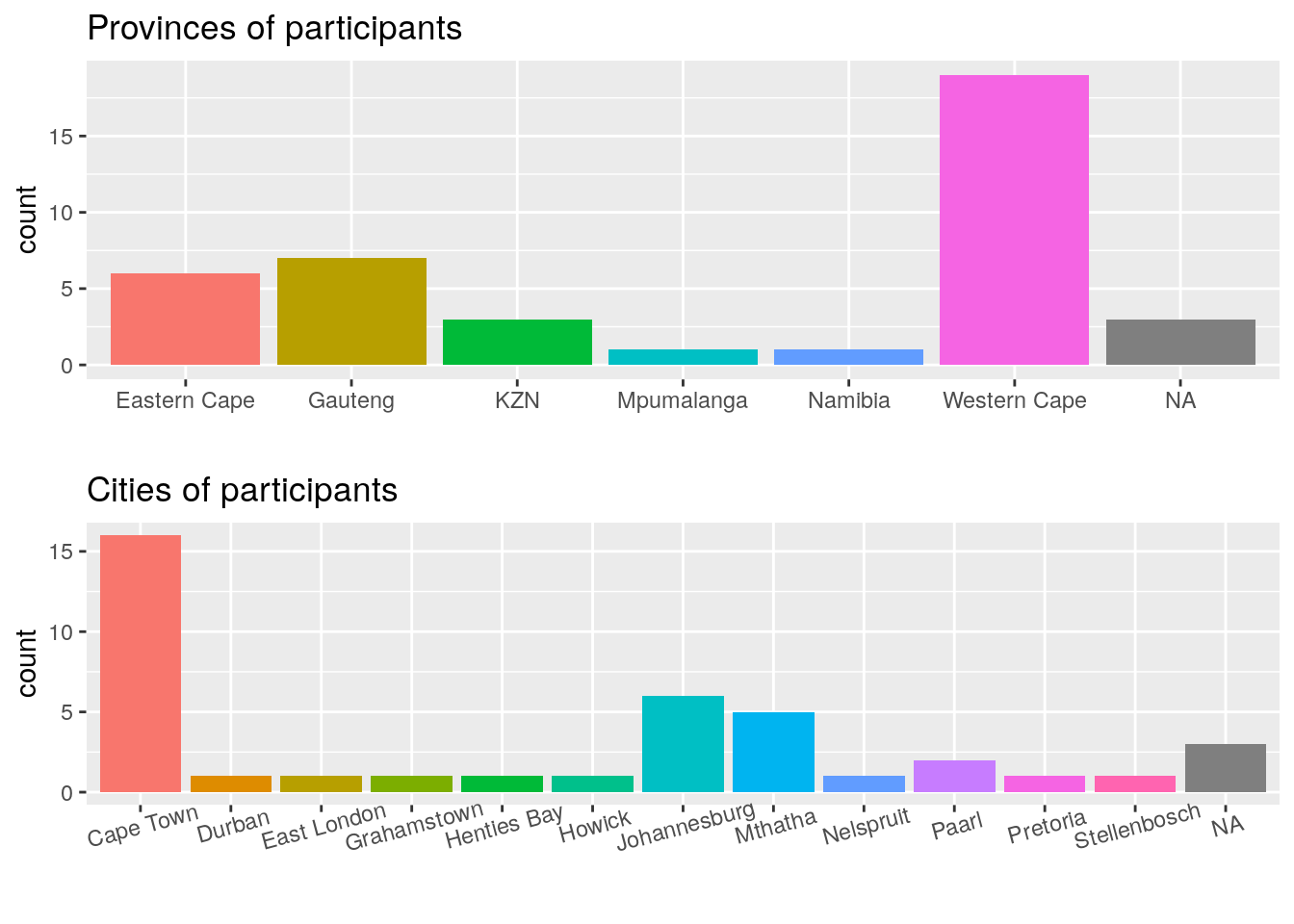
With our data prepared, I first wanted to see from where the surveys were taken. I’ve done this by splitting them up into province or city. This is also one of the few situations in which a bar plot is an appropriate visualisation. The columns below that show ‘NA’ are for participants that declined to share their location.
province_plot <- ggplot(data = survey, aes(x = province)) +
  geom_bar(aes(fill = province), show.legend = F) +
  ggtitle("Provinces of participants") +
  labs(x = "")
# province_plot
city_plot <- ggplot(data = survey, aes(x = city)) +
  geom_bar(aes(fill = city), show.legend = F) +
  ggtitle("Cities of participants") +
  labs(x = "") +
  theme(axis.text.x = element_text(angle = 15))
# city_plot
ggarrange(province_plot, city_plot, ncol = 1, nrow = 2)

Figure 1: Bar plots showing the total pariticpants by province or city.
Participant time frames
With the locations of of our participants visualised we now want to see what sort of time frames people around the country attribute to the three most common idioms.
ggplot(data = survey_long, aes(x = saying, y = minutes, fill = saying)) +
  geom_boxplot(show.legend = FALSE, outlier.colour = NA) +
  geom_jitter(shape = 21, alpha = 0.6, width = 0.3, height = 0.0, show.legend = FALSE) +
  scale_y_continuous(breaks = c(5, 15, 30, 60, 120, 300)) +
  scale_fill_brewer(palette = "Accent") +
  labs(x = "")

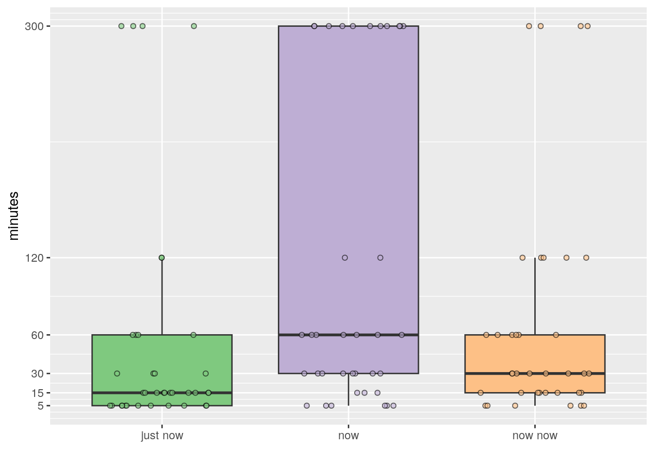
Figure 2: Boxplots showing the distribution of times (minutes) survey participants gave for the three most common time frame idioms in South Africa.
As we may see in Figure 2, ‘just now’ and ‘now now’ appear to have similar distributions, whereas ‘now’ is markedly different. Participants answered the maximum score of 300 minutes for all idioms, but for ‘just now’ and ‘now now’ this was infrequent enough that the large scores are considered to be outliers. For ‘now’, enough participants answered with longer times that the distribution appears much larger than for the other two idioms. Even though these distributions appear different, let’s run the stats on them to make sure. Because we want to compare distributions of scores for three different categories we will be using an ANOVA if the data meet a few basic assumptions.
Just as a quick recap, these assumptions are: homoscedasticity (homogeneity of variance), normality of distribution, random & independently sampled. It is also a good idea to have at least a sample size of ten for each category. Seeing as how this was an Internet survey, we were not able to ensure that the participants are a random representation of the South African populace, nor can we be certain that they submitted their answers independent of one another. I am however just going to go ahead and assume that they did. As for the assumptions of homoscedasticity and the normality of the distributions, we can directly test these. In R, the normality of a distribution is tested with shapiro.test(). Any non-significant result (p > 0.05) means that the data are normally distributed. To test for homoscedasticity we will use bartlett.test(). A non-significant result (p > 0.05) from this test indicates that the variances between the categories are equivalent.
# test for normality
survey_long %>%
  group_by(saying) %>%
  summarise(noramlity = as.numeric(shapiro.test(minutes)[1]))
## # A tibble: 3 × 2
##   saying   noramlity
##   <chr>        <dbl>
## 1 just now     0.565
## 2 now          0.713
## 3 now now      0.671
# Test for homoscedasticity
survey_long %>%
  bartlett.test(minutes ~ saying, data = .)
##
## 	Bartlett test of homogeneity of variances
##
## data:  minutes by saying
## Bartlett's K-squared = 5.227, df = 2, p-value = 0.07328
Surprisingly these data meet all of our assumptions so we may perform a simple one-way ANOVA on them to detect any significant differences.
glance(aov(minutes ~ saying, data = survey_long))
## # A tibble: 1 × 6
##   logLik   AIC   BIC deviance  nobs r.squared
##    <dbl> <dbl> <dbl>    <dbl> <int>     <dbl>
## 1  -670. 1349. 1360. 1143843.   111    0.0615
Less surprisingly, there is a significant difference in the times given for these three idioms. But let’s dive just a bit deeper with a post-hoc Tukey (not Turkey) test to see which categories specifically are different from which.
TukeyHSD(aov(minutes ~ saying, data = survey_long))
##   Tukey multiple comparisons of means
##     95% family-wise confidence level
##
## Fit: aov(formula = minutes ~ saying, data = survey_long)
##
## $saying
##                       diff         lwr       upr     p adj
## now-just now      60.81081    3.949653 117.67197 0.0330869
## now now-just now  14.18919  -42.671969  71.05035 0.8241544
## now now-now      -46.62162 -103.482779  10.23954 0.1302148
Looking at the names given in the ‘saying’ column, and the values given in the ‘p adj’ column we may see which individual idioms are different from which. Unsurprisingly, judging from Figure 2, ‘now now’ and ‘just now’ are not different. Interesting though is that ‘now’ is significantly different from ‘just now’, but not ‘now now’. The initial results made it look as though ‘now’ would have been significantly different from both.
Province time frames
Preferably, many more people would have taken the survey so that we could draw more conclusive results. I’m rather certain that should more people take the survey the distributions of the scores for the three idioms would even out more until there were no significant differences between any of them. Enough participants have taken the test however that we may compare the results for a few different provinces.
# Remove provinces with fewer than nine entries
# Ten would be preferable, but at nine we allow the inclusion of KZN
survey_province <- survey_long %>%
  group_by(province) %>%
  filter(n() >= 9) %>%
  ungroup()
And now with the provinces that have only a few answers filtered out, let’s see what the data look like as boxplots.
ggplot(data = survey_province, aes(x = saying, y = minutes, fill = province)) +
  geom_boxplot(outlier.colour = NA) +
  geom_point(shape = 21, position = position_jitterdodge()) +
  scale_y_continuous(breaks = c(5, 15, 30, 60, 120, 300)) +
  scale_fill_brewer(palette = "Set2") +
  labs(x = "")

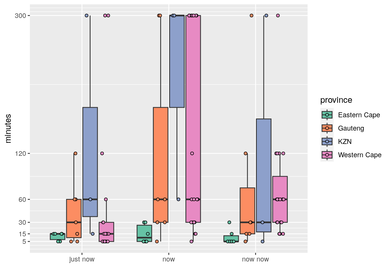
Figure 3: Boxplots showing the distribution of times by province.
Right away for me it appears that the time frames for the Eastern Cape are shorter than for the other three provinces. KZN appears to be the longest, with Gauteng and the Western Cape seeming similar. Because we have multiple independent variables (saying and province) we want a two-way ANOVA. But before we do that, let’s again check for normality and homoscedasticity.
# test for normality
survey_province %>%
  group_by(saying, province) %>%
  summarise(normality = as.numeric(shapiro.test(minutes)[1]))
## # A tibble: 12 × 3
## # Groups:   saying [3]
##    saying   province     normality
##    <chr>    <fct>            <dbl>
##  1 just now Eastern Cape     0.640
##  2 just now Gauteng          0.867
##  3 just now KZN              0.865
##  4 just now Western Cape     0.537
##  5 now      Eastern Cape     0.766
##  6 now      Gauteng          0.721
##  7 now      KZN              0.75
##  8 now      Western Cape     0.729
##  9 now now  Eastern Cape     0.684
## 10 now now  Gauteng          0.689
## 11 now now  KZN              0.813
## 12 now now  Western Cape     0.718
# Test for homoscedasticity
survey_province %>%
  bartlett.test(minutes ~ interaction(saying, province), data = .)
##
## 	Bartlett test of homogeneity of variances
##
## data:  minutes by interaction(saying, province)
## Bartlett's K-squared = 69.523, df = 11, p-value = 1.505e-10
The different groups of time are all normally distributed, but the variances differ. Regardless, we are going to stick to a normal two-way ANOVA as there are no good alternatives to this for non-parametric data and transforming these data is a bother.
glance(aov(minutes ~ saying + province, data = survey_province))
## # A tibble: 1 × 6
##   logLik   AIC   BIC deviance  nobs r.squared
##    <dbl> <dbl> <dbl>    <dbl> <int>     <dbl>
## 1  -623. 1261. 1279.  881685.   105     0.204
Significant differences are to be had here. So let’s break it down and see which groups specifically differ.
TukeyHSD(aov(minutes ~ saying + province, data = survey_province))
##   Tukey multiple comparisons of means
##     95% family-wise confidence level
##
## Fit: aov(formula = minutes ~ saying + province, data = survey_province)
##
## $saying
##                       diff        lwr        upr     p adj
## now-just now      70.14286   16.46427 123.821448 0.0068600
## now now-just now  15.42857  -38.25002  69.107162 0.7734013
## now now-now      -54.71429 -108.39288  -1.035695 0.0447008
##
## $province
##                                 diff         lwr       upr     p adj
## Gauteng-Eastern Cape       63.452381  -15.761193 142.66595 0.1624466
## KZN-Eastern Cape          139.722222   39.043527 240.40092 0.0025348
## Western Cape-Eastern Cape  73.289474    6.613379 139.96557 0.0252743
## KZN-Gauteng                76.269841  -21.982505 174.52219 0.1845631
## Western Cape-Gauteng        9.837093  -53.115472  72.78966 0.9768852
## Western Cape-KZN          -66.432749 -154.888584  22.02309 0.2092492
We may see that by removing some of the answers from the less represented provinces there is now a significant difference between the scores for ‘now’ and ‘now now’ as well as ‘just now’. Additionally we may see that the scores for Eastern Cape differ significantly from KZN and the Western Cape. One could also look at the interactions between the two independent variables but I’m not quite interested in that level of depth here.
City time frames
With the breakdown for the province time frames out of the way, we are going to wrap up this analysis by looking at the difference between cities.
# Remove provinces with fewer than five entries
# Ten is preferable, but at five we may include Mthatha
survey_city <- survey_long %>%
  group_by(saying, city) %>%
  filter(n() >= 5) %>%
  ungroup()
ggplot(data = survey_city, aes(x = saying, y = minutes, fill = city)) +
  geom_boxplot(outlier.colour = NA) +
  geom_point(shape = 21, position = position_jitterdodge()) +
  scale_y_continuous(breaks = c(5, 15, 30, 60, 120, 300)) +
  scale_fill_brewer(palette = "Set3") +
  labs(x = "")

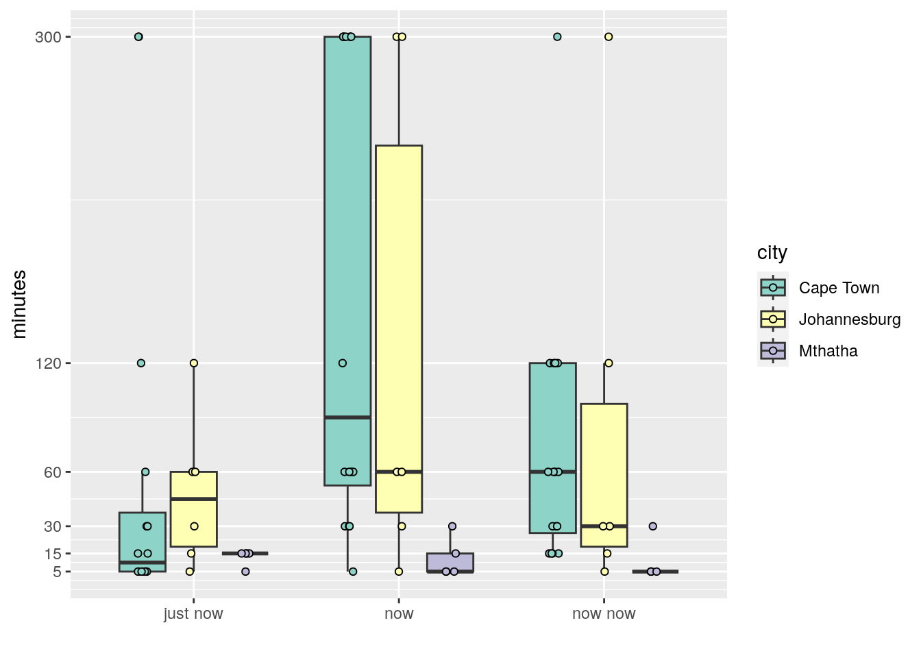
Figure 4: Boxplots showing the distribution of times by city.
Again with the assumptions…
# test for normality
survey_city %>%
  group_by(saying, city) %>%
  summarise(normality = as.numeric(shapiro.test(minutes)[1]))
## # A tibble: 9 × 3
## # Groups:   saying [3]
##   saying   city         normality
##   <chr>    <fct>            <dbl>
## 1 just now Cape Town        0.577
## 2 just now Johannesburg     0.912
## 3 just now Mthatha          0.552
## 4 now      Cape Town        0.739
## 5 now      Johannesburg     0.757
## 6 now      Mthatha          0.754
## 7 now now  Cape Town        0.739
## 8 now now  Johannesburg     0.741
## 9 now now  Mthatha          0.552
# Test for homoscedasticity
survey_city %>%
  bartlett.test(minutes ~ interaction(saying, city), data = .)
##
## 	Bartlett test of homogeneity of variances
##
## data:  minutes by interaction(saying, city)
## Bartlett's K-squared = 55.177, df = 8, p-value = 4.078e-09
… and again we see that while normally distributed, the variance of our sample sets differ significantly from one another. Regardless, we’ll stick to the two-way ANOVA.
glance(aov(minutes ~ saying + city, data = survey_city))
## # A tibble: 1 × 6
##   logLik   AIC   BIC deviance  nobs r.squared
##    <dbl> <dbl> <dbl>    <dbl> <int>     <dbl>
## 1  -481.  973.  987.  674933.    81     0.205
As one likely would have deduced from Figure 4, the scores are significantly different from one another.
TukeyHSD(aov(minutes ~ saying + city, data = survey_city))
##   Tukey multiple comparisons of means
##     95% family-wise confidence level
##
## Fit: aov(formula = minutes ~ saying + city, data = survey_city)
##
## $saying
##                       diff        lwr         upr     p adj
## now-just now      77.96296   16.65151 139.2744119 0.0090081
## now now-just now  16.85185  -44.45960  78.1633008 0.7889537
## now now-now      -61.11111 -122.42256   0.2003379 0.0509401
##
## $city
##                             diff        lwr        upr     p adj
## Johannesburg-Cape Town -10.72917  -72.99124  51.532904 0.9108240
## Mthatha-Cape Town      -84.89583 -151.53238 -18.259285 0.0088590
## Mthatha-Johannesburg   -74.16667 -152.92265   4.589316 0.0691761
From the post-hoc test we may see that ‘now’ differs significantly from ‘just now in these three cities, and if we’re feeling generous we may say that ‘now’ also differs significantly from ‘now now’. But like with the rest of the country, ‘now now’ and ‘just now’ are not significantly different time frames. Looking at the city breakdown we see that the only significant difference is between Mthatha and Cape Town. Johannesburg and Cape Town do not differ.
Conclusion
The general conclusion I’ve drawn from the analysis of the South Africa time survey results is that the understanding people in the Eastern Cape have of the time frames for these idioms is significantly faster than in the other major provinces in South Africa. The numbers don’t lie!
Speaking to people about this survey (before the results were out), the general consensus was that Johannesburg people would give significantly faster scores than people in other parts of the country, particularly Cape Town. That does not however appear to be the case. Also surprising from these results was that ‘now’ tended to be considered to be a significantly longer time frame than ‘just now’ and ‘now now’. Most people I’ve talked to about these idioms agree that ‘now’ is meant to be the fastest… so I’m not sure how that worked out. Unsurprising to me, but perhaps to some South Africans, was that there is no difference between ‘just now’ and ‘now now’. I was not surprised by this because talking with people around the country I very infrequently heard people, even while in the same room, agree on the time frames for these idioms.
There are of course a host of issues with this study. One thing I’m wondering about the Eastern Cape scores being significantly faster than the other provinces is if perhaps people in the Eastern Cape have a wider range of idioms for giving someone a time frame? Meaning, perhaps ‘now’, ‘just now’, and ‘now now’ are all much faster than other provinces because there is some other popular idiom people use there that denotes a longer time frame. It’s also possible that people in other provinces misunderstood the survey. Though I did make it very clear that the answers were in minutes and not seconds, specifically to attempt to prevent people from making that mistake. Lastly, this analysis suffers from a regrettably small sample size. I would have preferred at least 100 responses, rather than 40. It is still wonderful to be able to get some numbers in the game and get a glimpse of the fact that there is little agreement about these time frames.
Hopefully posting these results will snare a few more people into taking the survey and in another couple of months I can make a follow up post with the additional feedback.